import pandas as pd
import numpy as np
import matplotlib.pyplot as plt
from matplotlib.colors import ListedColormap
# Pour modifier la taille de sortie de graphiques dans le notebook
plt.rcParams['figure.figsize'] = [12, 12]
# Pour le traitement des données
from sklearn.preprocessing import StandardScaler
# le kNN et les SVM
from sklearn.neighbors import KNeighborsClassifier
from sklearn.svm import SVC
# Pour la CV
from sklearn.model_selection import train_test_split, GridSearchCV
file_path = "drive/MyDrive/Colab Notebooks/ml_data/TP4/Social_Network_Ads.csv"
data = pd.read_csv(file_path)
data| User ID | Gender | Age | EstimatedSalary | Purchased | |
|---|---|---|---|---|---|
| 0 | 15624510 | Male | 19 | 19000 | 0 |
| 1 | 15810944 | Male | 35 | 20000 | 0 |
| 2 | 15668575 | Female | 26 | 43000 | 0 |
| 3 | 15603246 | Female | 27 | 57000 | 0 |
| 4 | 15804002 | Male | 19 | 76000 | 0 |
| ... | ... | ... | ... | ... | ... |
| 395 | 15691863 | Female | 46 | 41000 | 1 |
| 396 | 15706071 | Male | 51 | 23000 | 1 |
| 397 | 15654296 | Female | 50 | 20000 | 1 |
| 398 | 15755018 | Male | 36 | 33000 | 0 |
| 399 | 15594041 | Female | 49 | 36000 | 1 |
400 rows × 5 columns
# On transforme la variable age en numérique
data["Gender"].replace(["Male", "Female"], [0, 1], inplace=True)
# On standardise et sauve les entrées
inputs = StandardScaler().fit_transform(data.drop(["User ID", "Purchased"], axis=1))
# On prend la sortie
outputs = data["Purchased"]
# On sépare le jeu de données
inputs_train_val, inputs_test, outputs_train_val, outputs_test \
  = train_test_split(inputs, outputs, test_size=0.25, stratify=outputs)
# Paramètres pour le nombre de voisins
k_par = list(range(1, 31))
param_dict = {"n_neighbors": k_par}
n_cv = 4
# Recherche sur grille avec CV
knn_classifier = KNeighborsClassifier()
gride_search_knn = GridSearchCV(knn_classifier,
param_dict,
cv=n_cv)
gride_search_knn.fit(inputs_train_val, outputs_train_val)GridSearchCV(cv=4, estimator=KNeighborsClassifier(),
param_grid={'n_neighbors': [1, 2, 3, 4, 5, 6, 7, 8, 9, 10, 11, 12,
13, 14, 15, 16, 17, 18, 19, 20, 21, 22,
23, 24, 25, 26, 27, 28, 29, 30]})In a Jupyter environment, please rerun this cell to show the HTML representation or trust the notebook. On GitHub, the HTML representation is unable to render, please try loading this page with nbviewer.org.
GridSearchCV(cv=4, estimator=KNeighborsClassifier(),
             param_grid={'n_neighbors': [1, 2, 3, 4, 5, 6, 7, 8, 9, 10, 11, 12,
                                         13, 14, 15, 16, 17, 18, 19, 20, 21, 22,
23, 24, 25, 26, 27, 28, 29, 30]})KNeighborsClassifier()
KNeighborsClassifier()
accuracy_knn_test = gride_search_knn.best_estimator_.score(inputs_test, outputs_test)
best_k = gride_search_knn.best_params_["n_neighbors"]
print(f"kNN: meilleure paramètre k = {best_k}")
print(f"kNN: meilleure exactitude d'entrainement = "
      f"{gride_search_knn.best_score_: .2%}")
print(f"kNN: meilleure exactitude de test = {accuracy_knn_test: .2%}")
kNN: meilleure paramètre k = 13
kNN: meilleure exactitude d'entrainement = 91.67%
kNN: meilleure exactitude de test = 90.00%# Les dimensions que nous allons examiner
dim_list = [(0, 1), (0, 2), (1, 2)]
# La position des graphs dans le carré
pos_list = [(0, 0), (0, 1), (1, 0)]
# Nos couleurs
mesh_cmap = ListedColormap(["lightblue", "coral"])
points_cmap = ListedColormap(["blue", "red"])
# La taille de la mesh
mesh_size = 0.1
# On créée le graphique
fig, axs = plt.subplots(2, 2)
# On fait une boucle sur les dimensions
for i, dim in enumerate(dim_list):
# On restreint les données
X = inputs[:, dim]
# On fixe les limites
x_min, x_max = X[:, 0].min() - 1, X[:, 0].max() + 1
y_min, y_max = X[:, 1].min() - 1, X[:, 1].max() + 1
# On définit notre mesh
xx, yy = np.meshgrid(np.arange(x_min, x_max, mesh_size),
np.arange(y_min, y_max, mesh_size))
# On définit les inputs
new_values = np.c_[xx.ravel(), yy.ravel()]
grid_input = np.zeros((new_values.shape[0], inputs.shape[1]))
grid_input[:, dim] = new_values
# On fait les prédictions, que l'on transforme en valeurs numériques
grid_pred = gride_search_knn.best_estimator_.predict(grid_input)
grid_pred = grid_pred.reshape(xx.shape)
# On fait le graphique
axs[pos_list[i]].pcolormesh(xx, yy, grid_pred, cmap=mesh_cmap)
axs[pos_list[i]].scatter(X[:, 0], X[:, 1], c=outputs, cmap=points_cmap)
axs[pos_list[i]].set_title(f"kNN k = {best_k}, test accuracy = {accuracy_knn_test:.2%}, dim = {dim}")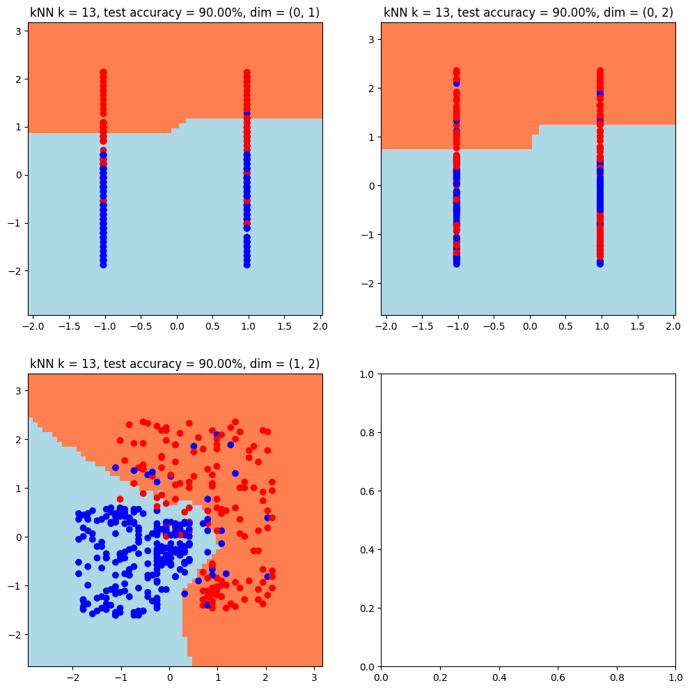
c_par = np.linspace(1, 10, 20)
gamma_par = np.linspace(0.01, 2, 20)
param_dict = {"C": c_par, "gamma": gamma_par}
n_cv = 4
svm_classifier = SVC()
# Recherche sur grille avec CV
gride_search_svm = GridSearchCV(svm_classifier,
                                param_dict,
                                cv=n_cv,
                                verbose=0)
gride_search_svm.fit(inputs_train_val, outputs_train_val)
GridSearchCV(cv=4, estimator=SVC(),
param_grid={'C': array([ 1. , 1.47368421, 1.94736842, 2.42105263, 2.89473684,
3.36842105, 3.84210526, 4.31578947, 4.78947368, 5.26315789,
5.73684211, 6.21052632, 6.68421053, 7.15789474, 7.63157895,
8.10526316, 8.57894737, 9.05263158, 9.52631579, 10. ]),
'gamma': array([0.01 , 0.11473684, 0.21947368, 0.32421053, 0.42894737,
0.53368421, 0.63842105, 0.74315789, 0.84789474, 0.95263158,
1.05736842, 1.16210526, 1.26684211, 1.37157895, 1.47631579,
1.58105263, 1.68578947, 1.79052632, 1.89526316, 2. ])})In a Jupyter environment, please rerun this cell to show the HTML representation or trust the notebook. On GitHub, the HTML representation is unable to render, please try loading this page with nbviewer.org.
GridSearchCV(cv=4, estimator=SVC(),
             param_grid={'C': array([ 1.        ,  1.47368421,  1.94736842,  2.42105263,  2.89473684,
        3.36842105,  3.84210526,  4.31578947,  4.78947368,  5.26315789,
        5.73684211,  6.21052632,  6.68421053,  7.15789474,  7.63157895,
        8.10526316,  8.57894737,  9.05263158,  9.52631579, 10.        ]),
                         'gamma': array([0.01      , 0.11473684, 0.21947368, 0.32421053, 0.42894737,
       0.53368421, 0.63842105, 0.74315789, 0.84789474, 0.95263158,
       1.05736842, 1.16210526, 1.26684211, 1.37157895, 1.47631579,
1.58105263, 1.68578947, 1.79052632, 1.89526316, 2. ])})SVC()
SVC()
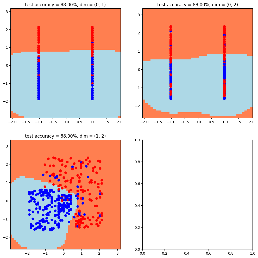
accuracy_svm_test = gride_search_svm.best_estimator_.score(inputs_test, outputs_test)
print(f"SVM: meilleures paramètres {gride_search_svm.best_params_}")
print(f"SVM: meilleure exactitude d'entrainement = "
      f"{gride_search_svm.best_score_: .2%}")
print(f"SVM: meilleure exactitude de test = {accuracy_svm_test: .2%}")
SVM: meilleures paramètres {'C': 1.4736842105263157, 'gamma': 0.9526315789473684}
SVM: meilleure exactitude d'entrainement = 92.33%
SVM: meilleure exactitude de test = 88.00%# On créée le graphique
fig, axs = plt.subplots(2, 2)
# On fait une boucle sur les dimensions
for i, dim in enumerate(dim_list):
# On restreint les données
X = inputs[:, dim]
# On fixe les limites
x_min, x_max = X[:, 0].min() - 1, X[:, 0].max() + 1
y_min, y_max = X[:, 1].min() - 1, X[:, 1].max() + 1
# On définit notre mesh
xx, yy = np.meshgrid(np.arange(x_min, x_max, mesh_size),
np.arange(y_min, y_max, mesh_size))
# On définit les inputs
new_values = np.c_[xx.ravel(), yy.ravel()]
grid_input = np.zeros((new_values.shape[0], inputs.shape[1]))
grid_input[:, dim] = new_values
# On fait les prédictions, que l'on transforme en valeurs numériques
grid_pred = gride_search_svm.best_estimator_.predict(grid_input)
grid_pred = grid_pred.reshape(xx.shape)
# On fait le graphique
axs[pos_list[i]].pcolormesh(xx, yy, grid_pred, cmap=mesh_cmap)
axs[pos_list[i]].scatter(X[:, 0], X[:, 1], c=outputs, cmap=points_cmap)
axs[pos_list[i]].set_title(f"test accuracy = {accuracy_svm_test:.2%}, "
f"dim = {dim}")