Machine Learning (Lettres) TP 1 : Prise en main

Les notebooks

Ce que vous avez devant les yeux est un Jupyter Notebook. C’est un rapport interactif, qui permet d’écrire du texte formaté (dans un langage de balises appelé Markdown, voir p.ex. https://www.markdowntutorial.com/) ainsi que du code Python, comme ci-dessous.

# Un exemple de code en Python
a = 10
b = 23
print(f"Le résultat de a + b est égal à {a + b}")

Le résultat de a + b est égal à 33

Vous devez normalement voir le résultat de votre sortie juste après le bloc de code. Remarquez que vous pouvez à tout moment modifier une partie du code pour changer son execution. (Faites le ! C’est en testant des choses que l’on apprend le mieux) Pour plus de détails à propros des Jupyter Notebooks https://docs.jupyter.org/en/latest/.

Les notebooks peuvent s’executer en local (sur votre machine, voir https://docs.jupyter.org/en/latest/install/notebook-classic.html), mais également sur un environnement d’execution distant (un serveur). Il existe plusieurs services proposant des serveurs pour des Jupyter Notebooks, p.ex. :

Google Colab: https://colab.research.google.com/
Paperspace Gradient : https://www.paperspace.com/gradient
Kaggle : https://www.kaggle.com/
Amazon SageMaker : https://aws.amazon.com/fr/sagemaker/

L’avantage des serveurs, c’est que l’installation (parfois fastidieuse) des différentes librairies Python est déjà faite, et qu’ils disposent de GPU (Graphical Processing Units) ou de TPU (Tensor Processing Units), utiles pour l’entrainement de nombreux modèles de Machine Learning.

Chargement et manipulation des données avec `pandas`

La première librairie python dont nous allons (re)voir l’utilisation est pandas https://pandas.pydata.org/, qui permet le chargement des fichiers de données ainsi que leur manipulation. On commence par la charger (on utilise fréquemment l’alias pd pour cette dernière).

import pandas as pd

Vérifiez que le chemin d’accès contenu dans file_path pointe bien sur le fichier “iris.csv” dans la première ligne de code de ce qui suit. Le chargement s’effectue ensuite facilement avec la fonction pd.read_csv(file_path) (il existe plusieurs options dans cette fonction pour, p.ex., changer le séparateur ou formater les variables).

file_path = "drive/MyDrive/Colab Notebooks/ml_data/TP1/iris.csv"
my_df = pd.read_csv(file_path)
my_df

	sepal.length	sepal.width	petal.length	petal.width	variety
0	5.1	3.5	1.4	0.2	Setosa
1	4.9	3.0	1.4	0.2	Setosa
2	4.7	3.2	1.3	0.2	Setosa
3	4.6	3.1	1.5	0.2	Setosa
4	5.0	3.6	1.4	0.2	Setosa
...	...	...	...	...	...
145	6.7	3.0	5.2	2.3	Virginica
146	6.3	2.5	5.0	1.9	Virginica
147	6.5	3.0	5.2	2.0	Virginica
148	6.2	3.4	5.4	2.3	Virginica
149	5.9	3.0	5.1	1.8	Virginica

150 rows × 5 columns

L’objet my_df est un objet de classe DataFrame.

type(my_df)

pandas.core.frame.DataFrame
def __init__(data=None, index: Axes | None=None, columns: Axes | None=None, dtype: Dtype | None=None, copy: bool | None=None) -> None

/usr/local/lib/python3.12/dist-packages/pandas/core/frame.pyTwo-dimensional, size-mutable, potentially heterogeneous tabular data.

Data structure also contains labeled axes (rows and columns).
Arithmetic operations align on both row and column labels. Can be
thought of as a dict-like container for Series objects. The primary
pandas data structure.

Parameters
----------
data : ndarray (structured or homogeneous), Iterable, dict, or DataFrame
    Dict can contain Series, arrays, constants, dataclass or list-like objects. If
    data is a dict, column order follows insertion-order. If a dict contains Series
    which have an index defined, it is aligned by its index. This alignment also
    occurs if data is a Series or a DataFrame itself. Alignment is done on
    Series/DataFrame inputs.

    If data is a list of dicts, column order follows insertion-order.

index : Index or array-like
    Index to use for resulting frame. Will default to RangeIndex if
    no indexing information part of input data and no index provided.
columns : Index or array-like
    Column labels to use for resulting frame when data does not have them,
    defaulting to RangeIndex(0, 1, 2, ..., n). If data contains column labels,
    will perform column selection instead.
dtype : dtype, default None
    Data type to force. Only a single dtype is allowed. If None, infer.
copy : bool or None, default None
    Copy data from inputs.
    For dict data, the default of None behaves like ``copy=True``.  For DataFrame
    or 2d ndarray input, the default of None behaves like ``copy=False``.
    If data is a dict containing one or more Series (possibly of different dtypes),
    ``copy=False`` will ensure that these inputs are not copied.

    .. versionchanged:: 1.3.0

See Also
--------
DataFrame.from_records : Constructor from tuples, also record arrays.
DataFrame.from_dict : From dicts of Series, arrays, or dicts.
read_csv : Read a comma-separated values (csv) file into DataFrame.
read_table : Read general delimited file into DataFrame.
read_clipboard : Read text from clipboard into DataFrame.

Notes
-----
Please reference the :ref:`User Guide <basics.dataframe>` for more information.

Examples
--------
Constructing DataFrame from a dictionary.

>>> d = {'col1': [1, 2], 'col2': [3, 4]}
>>> df = pd.DataFrame(data=d)
>>> df
   col1  col2
0     1     3
1     2     4

Notice that the inferred dtype is int64.

>>> df.dtypes
col1    int64
col2    int64
dtype: object

To enforce a single dtype:

>>> df = pd.DataFrame(data=d, dtype=np.int8)
>>> df.dtypes
col1    int8
col2    int8
dtype: object

Constructing DataFrame from a dictionary including Series:

>>> d = {'col1': [0, 1, 2, 3], 'col2': pd.Series([2, 3], index=[2, 3])}
>>> pd.DataFrame(data=d, index=[0, 1, 2, 3])
   col1  col2
0     0   NaN
1     1   NaN
2     2   2.0
3     3   3.0

Constructing DataFrame from numpy ndarray:

>>> df2 = pd.DataFrame(np.array([[1, 2, 3], [4, 5, 6], [7, 8, 9]]),
...                    columns=['a', 'b', 'c'])
>>> df2
   a  b  c
0  1  2  3
1  4  5  6
2  7  8  9

Constructing DataFrame from a numpy ndarray that has labeled columns:

>>> data = np.array([(1, 2, 3), (4, 5, 6), (7, 8, 9)],
...                 dtype=[("a", "i4"), ("b", "i4"), ("c", "i4")])
>>> df3 = pd.DataFrame(data, columns=['c', 'a'])
...
>>> df3
   c  a
0  3  1
1  6  4
2  9  7

Constructing DataFrame from dataclass:

>>> from dataclasses import make_dataclass
>>> Point = make_dataclass("Point", [("x", int), ("y", int)])
>>> pd.DataFrame([Point(0, 0), Point(0, 3), Point(2, 3)])
   x  y
0  0  0
1  0  3
2  2  3

Constructing DataFrame from Series/DataFrame:

>>> ser = pd.Series([1, 2, 3], index=["a", "b", "c"])
>>> df = pd.DataFrame(data=ser, index=["a", "c"])
>>> df
   0
a  1
c  3

>>> df1 = pd.DataFrame([1, 2, 3], index=["a", "b", "c"], columns=["x"])
>>> df2 = pd.DataFrame(data=df1, index=["a", "c"])
>>> df2
   x
a  1
c  3

Cet objet possède un index (pour lister les lignes), des noms de columns, et les types de ses variables.

print(my_df.index)
print(my_df.columns)
print(my_df.dtypes)

RangeIndex(start=0, stop=150, step=1)
Index(['sepal.length', 'sepal.width', 'petal.length', 'petal.width',
       'variety'],
      dtype='object')
sepal.length    float64
sepal.width     float64
petal.length    float64
petal.width     float64
variety          object
dtype: object

Il est possible d’accéder aux lignes et colonnes (variables) grâce à leur nom (Notez qu’ici, les lignes n’ont pas de nom, on utilise alors le “slicing”).

my_df["sepal.length"]

	sepal.length
0	5.1
1	4.9
2	4.7
3	4.6
4	5.0
...	...
145	6.7
146	6.3
147	6.5
148	6.2
149	5.9

150 rows × 1 columns

dtype: float64

my_df[1:3]

	sepal.length	sepal.width	petal.length	petal.width	variety
1	4.9	3.0	1.4	0.2	Setosa
2	4.7	3.2	1.3	0.2	Setosa

Notez qu’une colonne est un objet de la classe Series.

type(my_df["sepal.length"])

pandas.core.series.Series
def __init__(data=None, index=None, dtype: Dtype | None=None, name=None, copy: bool | None=None, fastpath: bool | lib.NoDefault=lib.no_default) -> None

/usr/local/lib/python3.12/dist-packages/pandas/core/series.pyOne-dimensional ndarray with axis labels (including time series).

Labels need not be unique but must be a hashable type. The object
supports both integer- and label-based indexing and provides a host of
methods for performing operations involving the index. Statistical
methods from ndarray have been overridden to automatically exclude
missing data (currently represented as NaN).

Operations between Series (+, -, /, \*, \*\*) align values based on their
associated index values-- they need not be the same length. The result
index will be the sorted union of the two indexes.

Parameters
----------
data : array-like, Iterable, dict, or scalar value
    Contains data stored in Series. If data is a dict, argument order is
    maintained.
index : array-like or Index (1d)
    Values must be hashable and have the same length as `data`.
    Non-unique index values are allowed. Will default to
    RangeIndex (0, 1, 2, ..., n) if not provided. If data is dict-like
    and index is None, then the keys in the data are used as the index. If the
    index is not None, the resulting Series is reindexed with the index values.
dtype : str, numpy.dtype, or ExtensionDtype, optional
    Data type for the output Series. If not specified, this will be
    inferred from `data`.
    See the :ref:`user guide <basics.dtypes>` for more usages.
name : Hashable, default None
    The name to give to the Series.
copy : bool, default False
    Copy input data. Only affects Series or 1d ndarray input. See examples.

Notes
-----
Please reference the :ref:`User Guide <basics.series>` for more information.

Examples
--------
Constructing Series from a dictionary with an Index specified

>>> d = {'a': 1, 'b': 2, 'c': 3}
>>> ser = pd.Series(data=d, index=['a', 'b', 'c'])
>>> ser
a   1
b   2
c   3
dtype: int64

The keys of the dictionary match with the Index values, hence the Index
values have no effect.

>>> d = {'a': 1, 'b': 2, 'c': 3}
>>> ser = pd.Series(data=d, index=['x', 'y', 'z'])
>>> ser
x   NaN
y   NaN
z   NaN
dtype: float64

Note that the Index is first build with the keys from the dictionary.
After this the Series is reindexed with the given Index values, hence we
get all NaN as a result.

Constructing Series from a list with `copy=False`.

>>> r = [1, 2]
>>> ser = pd.Series(r, copy=False)
>>> ser.iloc[0] = 999
>>> r
[1, 2]
>>> ser
0    999
1      2
dtype: int64

Due to input data type the Series has a `copy` of
the original data even though `copy=False`, so
the data is unchanged.

Constructing Series from a 1d ndarray with `copy=False`.

>>> r = np.array([1, 2])
>>> ser = pd.Series(r, copy=False)
>>> ser.iloc[0] = 999
>>> r
array([999,   2])
>>> ser
0    999
1      2
dtype: int64

Due to input data type the Series has a `view` on
the original data, so
the data is changed as well.

Plusieurs opérations sont possibles sur ce type d’objet.

my_df["sepal.length"] + my_df["sepal.width"]

	0
0	8.6
1	7.9
2	7.9
3	7.7
4	8.6
...	...
145	9.7
146	8.8
147	9.5
148	9.6
149	8.9

150 rows × 1 columns

dtype: float64

my_df["sepal.length"] < 5

	sepal.length
0	False
1	True
2	True
3	True
4	False
...	...
145	False
146	False
147	False
148	False
149	False

150 rows × 1 columns

dtype: bool

Ajouter une colonne à notre DataFrame est également très aisé.

my_df["sepal.length.cat"] = my_df["sepal.length"] < 5
my_df

	sepal.length	sepal.width	petal.length	petal.width	variety	sepal.length.cat
0	5.1	3.5	1.4	0.2	Setosa	False
1	4.9	3.0	1.4	0.2	Setosa	True
2	4.7	3.2	1.3	0.2	Setosa	True
3	4.6	3.1	1.5	0.2	Setosa	True
4	5.0	3.6	1.4	0.2	Setosa	False
...	...	...	...	...	...	...
145	6.7	3.0	5.2	2.3	Virginica	False
146	6.3	2.5	5.0	1.9	Virginica	False
147	6.5	3.0	5.2	2.0	Virginica	False
148	6.2	3.4	5.4	2.3	Virginica	False
149	5.9	3.0	5.1	1.8	Virginica	False

150 rows × 6 columns

Pour sélectionner plusieurs lignes et colonnes, on peut utiliser my_df.loc, qui va sélectionner en utilisant les labels.

my_df.loc[1:5, ["sepal.length", "sepal.length.cat"]]

	sepal.length	sepal.length.cat
1	4.9	True
2	4.7	True
3	4.6	True
4	5.0	False
5	5.4	False

Ou avec my_df.iloc pour faire des accessions avec des indices.

my_df.iloc[:, 3:5]

	petal.width	variety
0	0.2	Setosa
1	0.2	Setosa
2	0.2	Setosa
3	0.2	Setosa
4	0.2	Setosa
...	...	...
145	2.3	Virginica
146	1.9	Virginica
147	2.0	Virginica
148	2.3	Virginica
149	1.8	Virginica

150 rows × 2 columns

On peut égalament transformer un Dataframe en un objet numpy.ndarray, propice aux opérations mathématiques.

my_df.iloc[:, :4].to_numpy()

array([[5.1, 3.5, 1.4, 0.2],
       [4.9, 3. , 1.4, 0.2],
       [4.7, 3.2, 1.3, 0.2],
       [4.6, 3.1, 1.5, 0.2],
       [5. , 3.6, 1.4, 0.2],
       [5.4, 3.9, 1.7, 0.4],
       [4.6, 3.4, 1.4, 0.3],
       [5. , 3.4, 1.5, 0.2],
       [4.4, 2.9, 1.4, 0.2],
       [4.9, 3.1, 1.5, 0.1],
       [5.4, 3.7, 1.5, 0.2],
       [4.8, 3.4, 1.6, 0.2],
       [4.8, 3. , 1.4, 0.1],
       [4.3, 3. , 1.1, 0.1],
       [5.8, 4. , 1.2, 0.2],
       [5.7, 4.4, 1.5, 0.4],
       [5.4, 3.9, 1.3, 0.4],
       [5.1, 3.5, 1.4, 0.3],
       [5.7, 3.8, 1.7, 0.3],
       [5.1, 3.8, 1.5, 0.3],
       [5.4, 3.4, 1.7, 0.2],
       [5.1, 3.7, 1.5, 0.4],
       [4.6, 3.6, 1. , 0.2],
       [5.1, 3.3, 1.7, 0.5],
       [4.8, 3.4, 1.9, 0.2],
       [5. , 3. , 1.6, 0.2],
       [5. , 3.4, 1.6, 0.4],
       [5.2, 3.5, 1.5, 0.2],
       [5.2, 3.4, 1.4, 0.2],
       [4.7, 3.2, 1.6, 0.2],
       [4.8, 3.1, 1.6, 0.2],
       [5.4, 3.4, 1.5, 0.4],
       [5.2, 4.1, 1.5, 0.1],
       [5.5, 4.2, 1.4, 0.2],
       [4.9, 3.1, 1.5, 0.2],
       [5. , 3.2, 1.2, 0.2],
       [5.5, 3.5, 1.3, 0.2],
       [4.9, 3.6, 1.4, 0.1],
       [4.4, 3. , 1.3, 0.2],
       [5.1, 3.4, 1.5, 0.2],
       [5. , 3.5, 1.3, 0.3],
       [4.5, 2.3, 1.3, 0.3],
       [4.4, 3.2, 1.3, 0.2],
       [5. , 3.5, 1.6, 0.6],
       [5.1, 3.8, 1.9, 0.4],
       [4.8, 3. , 1.4, 0.3],
       [5.1, 3.8, 1.6, 0.2],
       [4.6, 3.2, 1.4, 0.2],
       [5.3, 3.7, 1.5, 0.2],
       [5. , 3.3, 1.4, 0.2],
       [7. , 3.2, 4.7, 1.4],
       [6.4, 3.2, 4.5, 1.5],
       [6.9, 3.1, 4.9, 1.5],
       [5.5, 2.3, 4. , 1.3],
       [6.5, 2.8, 4.6, 1.5],
       [5.7, 2.8, 4.5, 1.3],
       [6.3, 3.3, 4.7, 1.6],
       [4.9, 2.4, 3.3, 1. ],
       [6.6, 2.9, 4.6, 1.3],
       [5.2, 2.7, 3.9, 1.4],
       [5. , 2. , 3.5, 1. ],
       [5.9, 3. , 4.2, 1.5],
       [6. , 2.2, 4. , 1. ],
       [6.1, 2.9, 4.7, 1.4],
       [5.6, 2.9, 3.6, 1.3],
       [6.7, 3.1, 4.4, 1.4],
       [5.6, 3. , 4.5, 1.5],
       [5.8, 2.7, 4.1, 1. ],
       [6.2, 2.2, 4.5, 1.5],
       [5.6, 2.5, 3.9, 1.1],
       [5.9, 3.2, 4.8, 1.8],
       [6.1, 2.8, 4. , 1.3],
       [6.3, 2.5, 4.9, 1.5],
       [6.1, 2.8, 4.7, 1.2],
       [6.4, 2.9, 4.3, 1.3],
       [6.6, 3. , 4.4, 1.4],
       [6.8, 2.8, 4.8, 1.4],
       [6.7, 3. , 5. , 1.7],
       [6. , 2.9, 4.5, 1.5],
       [5.7, 2.6, 3.5, 1. ],
       [5.5, 2.4, 3.8, 1.1],
       [5.5, 2.4, 3.7, 1. ],
       [5.8, 2.7, 3.9, 1.2],
       [6. , 2.7, 5.1, 1.6],
       [5.4, 3. , 4.5, 1.5],
       [6. , 3.4, 4.5, 1.6],
       [6.7, 3.1, 4.7, 1.5],
       [6.3, 2.3, 4.4, 1.3],
       [5.6, 3. , 4.1, 1.3],
       [5.5, 2.5, 4. , 1.3],
       [5.5, 2.6, 4.4, 1.2],
       [6.1, 3. , 4.6, 1.4],
       [5.8, 2.6, 4. , 1.2],
       [5. , 2.3, 3.3, 1. ],
       [5.6, 2.7, 4.2, 1.3],
       [5.7, 3. , 4.2, 1.2],
       [5.7, 2.9, 4.2, 1.3],
       [6.2, 2.9, 4.3, 1.3],
       [5.1, 2.5, 3. , 1.1],
       [5.7, 2.8, 4.1, 1.3],
       [6.3, 3.3, 6. , 2.5],
       [5.8, 2.7, 5.1, 1.9],
       [7.1, 3. , 5.9, 2.1],
       [6.3, 2.9, 5.6, 1.8],
       [6.5, 3. , 5.8, 2.2],
       [7.6, 3. , 6.6, 2.1],
       [4.9, 2.5, 4.5, 1.7],
       [7.3, 2.9, 6.3, 1.8],
       [6.7, 2.5, 5.8, 1.8],
       [7.2, 3.6, 6.1, 2.5],
       [6.5, 3.2, 5.1, 2. ],
       [6.4, 2.7, 5.3, 1.9],
       [6.8, 3. , 5.5, 2.1],
       [5.7, 2.5, 5. , 2. ],
       [5.8, 2.8, 5.1, 2.4],
       [6.4, 3.2, 5.3, 2.3],
       [6.5, 3. , 5.5, 1.8],
       [7.7, 3.8, 6.7, 2.2],
       [7.7, 2.6, 6.9, 2.3],
       [6. , 2.2, 5. , 1.5],
       [6.9, 3.2, 5.7, 2.3],
       [5.6, 2.8, 4.9, 2. ],
       [7.7, 2.8, 6.7, 2. ],
       [6.3, 2.7, 4.9, 1.8],
       [6.7, 3.3, 5.7, 2.1],
       [7.2, 3.2, 6. , 1.8],
       [6.2, 2.8, 4.8, 1.8],
       [6.1, 3. , 4.9, 1.8],
       [6.4, 2.8, 5.6, 2.1],
       [7.2, 3. , 5.8, 1.6],
       [7.4, 2.8, 6.1, 1.9],
       [7.9, 3.8, 6.4, 2. ],
       [6.4, 2.8, 5.6, 2.2],
       [6.3, 2.8, 5.1, 1.5],
       [6.1, 2.6, 5.6, 1.4],
       [7.7, 3. , 6.1, 2.3],
       [6.3, 3.4, 5.6, 2.4],
       [6.4, 3.1, 5.5, 1.8],
       [6. , 3. , 4.8, 1.8],
       [6.9, 3.1, 5.4, 2.1],
       [6.7, 3.1, 5.6, 2.4],
       [6.9, 3.1, 5.1, 2.3],
       [5.8, 2.7, 5.1, 1.9],
       [6.8, 3.2, 5.9, 2.3],
       [6.7, 3.3, 5.7, 2.5],
       [6.7, 3. , 5.2, 2.3],
       [6.3, 2.5, 5. , 1.9],
       [6.5, 3. , 5.2, 2. ],
       [6.2, 3.4, 5.4, 2.3],
       [5.9, 3. , 5.1, 1.8]])

Bien entendu, il existe encore de nombreuses fonctionnalités dans pandas. Pour en savoir plus, la communauté propose de nombreux tutoriels https://pandas.pydata.org/docs/getting_started/tutorials.html.

Opérations mathématiques avec `numpy`

La librairie numpy https://numpy.org/ est la référence pour tout ce qui est opérations mathématiques et est utilisé de manière quasiment systématique dans tout projet de Machine Learning. On l’importe fréquemment sous l’alias np.

import numpy as np

Les objets essentiels dans numpy, permettant de représenter les vecteurs ou les matrices, sont les Arrays (numpy.array). Elles peuvent être créées à partir de listes (ou listes de listes pour un tableau).

a = np.array([1, 2, 3, 4, 5, 6])
b = np.array([[1, 2, 3, 4],
              [5, 6, 7, 8],
              [9, 10, 11, 12]])
a

array([1, 2, 3, 4, 5, 6])

array([[ 1,  2,  3,  4],
       [ 5,  6,  7,  8],
       [ 9, 10, 11, 12]])

On peut obtenir plusieurs information sur une Array.

a.ndim # Combien d'axes

b.size # Combien d'éléments

b.shape # Sa forme

(3, 4)

a.shape

(6,)

b.dtype # Le type de ses éléments

dtype('int64')

Les crochets permettent l’accession et la modification.

b[[0, 2], :3]

array([[ 1,  2,  3],
       [ 9, 10, 11]])

b[0, 0] = 100
b

array([[100,   2,   3,   4],
       [  5,   6,   7,   8],
       [  9,  10,  11,  12]])

Il est aussi possible de les redimmensionner les Arrays,

c = b.reshape([2, 6])
c

array([[100,   2,   3,   4,   5,   6],
       [  7,   8,   9,  10,  11,  12]])

de les transposer,

c.T

array([[100,   7],
       [  2,   8],
       [  3,   9],
       [  4,  10],
       [  5,  11],
       [  6,  12]])

et de faire de nombreuses opérations mathématiques sur ces dernières. Les opérateurs classiques agissent sur chaque élément.

b / 10

array([[10. ,  0.2,  0.3,  0.4],
       [ 0.5,  0.6,  0.7,  0.8],
       [ 0.9,  1. ,  1.1,  1.2]])

print(c)
print(a)

[[100   2   3   4   5   6]
 [  7   8   9  10  11  12]]
[1 2 3 4 5 6]

print(c.shape)
print(a.shape)
c + a # L'objet le plus petit (a) est dupliqué pour avoir une taille suffisante

(2, 6)
(6,)

array([[101,   4,   6,   8,  10,  12],
       [  8,  10,  12,  14,  16,  18]])

np.cos(a)

array([ 0.54030231, -0.41614684, -0.9899925 , -0.65364362,  0.28366219,
        0.96017029])

L’opérateur @ effectue la multiplication matricielle.

e = np.array([1, 10, 100, 1000])
b @ e

array([ 4420,  8765, 13209])

b est (3 x 4), e est (4 x 1), l’opération est donc valide et le résultat est bien de dimension (3 x 1).

Il existe encore de nombreuses fonctionnalités dans numpy, pour voir plus loin https://numpy.org/doc/stable/user/whatisnumpy.html.

Graphiques avec `matplotlib`

La dernière librairie que nous allons voir aujourd’hui est matplotlib https://matplotlib.org/, qui permet l’affichage de nombreux types de graphiques. On importe généralement uniquement son module pyplot avec l’alias plt.

import matplotlib.pyplot as plt

Cette librairie est longue à prendre en main et nous n’avons malheureusement pas le temps de la voir en détail. Nous verrons de nombreux exemples d’utilisation durant ce cours ce qui permettra de voir son fonctionnement. Par exemple, pour faire un nuage de points (scatterplot) de nos Iris, on peut faire :

# Création d'un dictionnaire pour les couleurs
colors = {"Setosa": "blue", "Versicolor": "green", "Virginica": "red"}

# Création des objets servant à l'affichage graphique
fig, ax = plt.subplots()

# On fait une boucle sur les espèces
for species in my_df["variety"].unique():

  # Selection de l'espèce
  species_df = my_df[my_df["variety"] == species]

  # Scatter plot de l'espèce
  ax.scatter(x=species_df["sepal.length"],
            y=species_df["sepal.width"],
            c=colors[species],
            label=species)

# Ajout du nom des axes, d'un titre, d'une légende, et d'une grille
ax.set_xlabel("Sepal Length")
ax.set_ylabel("Sepal Width")
ax.set_title("Iris")
ax.legend()
ax.grid(True)

plt.plot()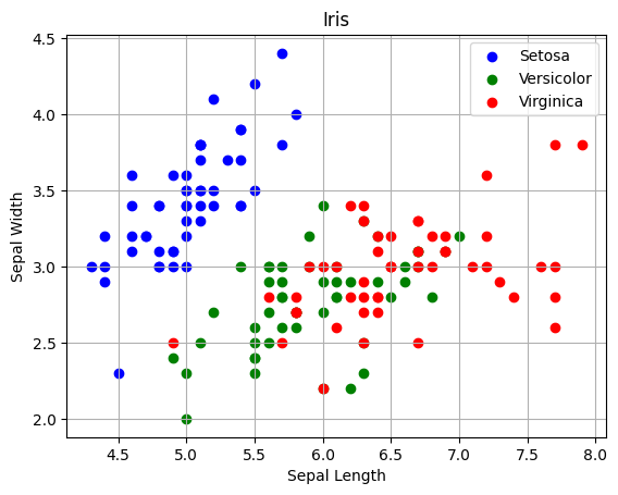

Si vous voulez une réelle prise en main, vous pouvez suivre les tutoriels à https://matplotlib.org/stable/tutorials/index.html.

Machine Learning (Lettres) TP 1 : Prise en main

Les notebooks

Chargement et manipulation des données avec pandas

Opérations mathématiques avec numpy

Graphiques avec matplotlib

Chargement et manipulation des données avec `pandas`

Opérations mathématiques avec `numpy`

Graphiques avec `matplotlib`